AI math handbook calculator - Fractional Calculus Computer Algebra System software

Drawing 画画

Do exercise and learn from example. If something wrong, please clear meomery by clicking the AC button, then do again.

Arithmetic 算术 >>

Exact computation

Fraction `1E2-1/2`

mod operation:
input mod(3,2) for 3 mod 2

big number in Java

Add prefix "big" to number for Big integer:
big1234567890123456789-1

Add prefix "big" to number for Big decimal:
big1.234567890123456789-1

big number in JavaScript

computation in JavaScript should to click the numeric button or expression ending with equal sign =

The default precision for BigNumber is 64 digits, and can be configured with the option precision.

bignumber(1.23456789123456789)=

Round-off errors

Calculations with BigNumber are much slower than calculations with Number, but they can be executed with an arbitrary precision. By using a higher precision, it is less likely that round-off errors occur:
// round-off errors with numbers

math.add(0.1, 0.2) // Number, 0.30000000000000004

math.divide(0.3, 0.2) // Number, 1.4999999999999998

// no round-off errors with BigNumbers :)

math.add(math.bignumber(0.1), math.bignumber(0.2)) // BigNumber, 0.3

math.divide(math.bignumber(0.3), math.bignumber(0.2)) // BigNumber, 1.5

Numerical approximations

There are two types of numeric computation: JavaScript and Java numeric computation:

JavaScript numeric computation

numeric computation with the ≈ button :
acos(bignumber(-1))

numeric computation end with the equal sign = :
acos(bignumber(-1))=

Java numeric computation

numeric computation with the ≈≈ button :
sin(pi/4)

Convert back with numeric computation function n(x) :
n(polar(2,45degree))
n( sin(pi/4) )
n( sin(30 degree) )

`sin^((0.5))(1)` is the 0.5 order derivative of sin(x) at x=1 :
n( sin(0.5,1) )

`sin(1)^(0.5)` is the 0.5 power of sin(x) at x=1 :
n( sin(1)^0.5 )

more are in numeric math

Complex 复数

math handbook chapter 1.1.2 complex
There are two types of complex number: JavaScript complex and Java complex:

input complex numbers

input complex numbers in the complex plane:
1+2i

in small letters of complex(1,2) is complex number:
complex(1,2)

in first upper case letter of Complex(1,2) is object in JavaScript complex:
Complex(1,2)

input complex number in polar(r,theta) coordinates:
polar(1,pi)

input complex number in polar(r,theta*degree) coordinates:
polar(1,45degree)

input complex number in polar(r,theta) coordinates for degree by polard(r,degree):
polard(1,45)

input complex number in trig format of r*cis(theta*degree) :
2cis(45degree)

Convert complex to polar(r,theta) coordinates

Convert complex a+b*i to polar(r,theta) coordinates in Java:
convert 1-i to polar
topolar(1-i)
convert back to a+b*i format by to remove last letter s or click the simplify button

Convert complex a+b*i to polar(r,theta*degree) coordinates:
topolard(1-i)

convert back to a+b*i format by to remove last letter s or click the simplify button

Convert complex a+b*i to polar(r,theta) coordinates in JavaScript:
math.Complex(1,2).toPolar()=
math.complex(1,2).toPolar()=

convert to vector

complex(1,2) number is special vector, i.e. the 2-dimentional vector, so it can be converted to vector.

to Java vector(1,2)
convert 1-i to vector
tovector(1-i)

to JavaScript vector [1,2]
math.Complex(1,2).toVector()=
math.complex(1,2).toVector()=

complex number plot

in order to auto plot complex number as vector, input complex(1,-2) for 1-2i, or convert 1-2i to complex(1,-2) by
convert 1-2i to complex
convert(1-2i to complex)
tocomplex(1-2i)

complex function plot

complex animation(z) show animation of complex function in complex domain of complex variable z.

complexplot(z) show phrase and/or modulus of complex function in complex domain of complex variable z.

re2D plot: real curve (blue) and imag cureve (red) on real domain
re2D(x^x)

im2D plot: real curve (blue) and imag cureve (red) on imag domain
im2D(x^x)

put imagary i with variable x for plot on imag domain:
exp(i*x)

more are in complex2D(x) show 2 curves of real and imag parts in realand imag domains.

complex 3D plot:
complex3D(pow(x,x))

more are in complex function with complex3D(x) in complex domain of complex variable x.

Numeric math 数值数学 >>

数值数学 = 计算数学
math handbook chapter 3.4

computation in JavaScript should to click the numeric button or expression ending with equal sign =
sin(pi/4)=

numeric computation with the n(x) ≈≈ button:
n( sin(30 degree) )
n sin(30 degree)

numeric solve equation:
nsolve( x^2-5*x+6=0 )
nsolve( x^2-5*x+6 )

find_root(x,-10,10) between -10 and 10 for numeric equation:
find_root( x^2-5*x+6==0 )
find_root( x^2-5*x+6 )

JavaScript numeric calculator with the ≈ button can calculate numeric, number theory, Probability, Statistics, matrix, solve equation.

more example in JavaScript mathjs

numeric integrate, by default x from 0 to 1:
nint( x^2-5*x+6,x,0,1 )
nint x^2-5*x+6 as x from 0 to 1
nint sin(x)

numeric computation with the funplot ≈ button:
integrate(x=>sin(x),[1,2])

more calculus operation in JavaScript calculus

Algebra 代数 >>

math handbook chapter 1 algebra

simplify:
taylor( (x^2 - 1)/(x-1) )

expand:
expand( (x-1)^3 )

factorizing:
factor( x^2+3*x+2 )

factor high order polymonial by factor(x)== :
factor( x^3-1 )==

factorization:
factor( x^4-1 )==

combine two terms:
combine( log(a)+log(b) )

tangent

tangent equation at x=0 by default
tangent( sin(x) )

tangent equation at x=1
tangent( sin(x),x=1 )

tangentplot(x) show dynamic tangent line when your mouse over the curve.
tangentplot( sin(x) )

convert

convert( sin(x) to exp) is the same as toexp(sin(x))

convert to exp:
toexp( cos(x) )

convert to trig:
convert exp(x) to trig

convert sin(x) to exp(x):
convert sin(x) to exp = toexp( sin(x) )

Convert to exp(x):
toexp(Gamma(2,x))

inverse function

input sin(x), click the inverse button
inverse( sin(x) )
check its result by clicking the inverse button again.
In order to show multi-value, use the inverse equation instead function.

inverse equation

inverse equation to show multivalue if it has:
inverse( sin(x)=y )
check its result by clicking the inverse button again.

polynomial

math handbook chapter 20.5 polynomial

the unit polynomial:
Enter poly(3,x) = poly(3) for the unit polynomial with degree 3: x^3+x^2+x+1.

Hermite polynomial:
hermite(3,x) gives the Hermite polynomial while hermite(3) gives Hermite number.

harmonic polynomial:
harmonic(-3,1,x) = harmonic(-3,x)

the zeta( ) polynomial:
zeta(-3,x)

simplify(x):
taylor( (x^2 - 1)/(x-1) )

expand(x) polynomial:
expand(hermite(3,x))

topoly(x) convert polynomial to polys(x) as holder of polynomial coefficients,
convert `x^2-5*x+6` to poly = topoly( `x^2-5*x+6` )

simplify polys(x) to polynomial:
simplify( polys(1,-5,6,x) )

polyroots(x) is holder of polynomial roots, topolyroot(x) convert a polynomial to polyroots.
convert (x^2-1) to polyroot = topolyroot(x^2-1)

polysolve(x) numerically solve polynomial for multi-roots:
polysolve(x^2-1)

nsolve(x) numerically solve for a single root:
nsolve(x^2-1)

solve(x) for sybmbloic and numeric roots:
solve(x^2-1)

construct polynomial from roots, activate polyroots(x) to polynomial, and reduce roots to polynomial equation = 0 by click on the simplify(x) button.
simplify( polyroots(2,3) )

Number

When the variable x of polynomial is numnber, it becomes polynomial number, please see Number_Theory section.

Function 函数 >>

math handbook chapter 1 Function 函数

Trigonometry 三角函数

expand Trigonometry by expandtrig(x) :
expandtrig( sin(x)^2 )

inverse function :
inverse( sin(x) )

plot a multivalue function by the inverse equation :
inverse( sin(x)=y )

expand trig function :
expandtrig( sin(x)^2 )

expand special function :
expand( gamma(2,x) )

factor(x) :
factor( sin(x)*cos(x) )

Complex Function 复变函数

math handbook chapter 10 Complex Function 复变函数
complex2D(x) shows 2 curves of the real and imag parts in real domain x, and complex3D(x) shows complex function in complex domain x, for 20 graphes in one plot.

re2D plot: real curve (blue) and imag cureve (red) on real domain
re2D(x^x)

im2D plot: real curve (blue) and imag cureve (red) on imag domain
im2D(x^x)

put imagary i with variable x for plot on imag domain:
exp(i*x)

more are in complex2D(x) for 2 curves of real and imag parts in complex domain of complex variable x.

complex animation(z) show animation of complex function in complex domain of complex variable z.

complexplot(z) show phrase and/or modulus of complex function in complex domain of complex variable z.

complex 3D plot :
complex3D(pow(x,x)) in complex domain of complex variable x.

Complex

complex - complex math - complex function

complex2D
1. complex animate(z) or complex2D(z) for phase animation in complex plane, the independent variable must be z.
2. complex plot(z) for phase and/or modulus in complex plane, the independent variable must be z.
3. plot complex(z) for phase and/or modulus in complex plane, the independent variable must be z.
4. re2D(x) and im2D(x) show for complex 2 curves of real and imag parts in real and imag domain, the independent variable must be x.
5. complex coloring
6. color WebXR surface of complex function on complex plane
complex3D
1. complex3D(x) for 3 dimensional graph, the independent variable must be x.
2. Riemann surface
3. Complex Branches

References

math handbook content 2 chapter 10 complex function
math handbook content 3 chapter 10 complex function
math handbook content 4 chapter 10 complex function
Complex analysis

more are in complex function

special Function

math handbook chapter 12 special Function

Calculus 微积分 >>

Limit

math handbook chapter 4.1 limit

click the lim(x) button for lim at x->0 :
`lim_(x->0) sin(x)/x ` = lim sin(x)/x as x->0 = lim(sin(x)/x)

click the nlim(x) button for numeric limit at x->0 :
nlim(sin(x)/x)

click the limit(x) button for limit at x->oo :
limi`t_(x->oo) log(x)/x` = limit( log(x)/x as x->inf )
= limoo( log(x)/x )

one side limit, left or right side :
lim(exp(-x),x,0,right)

Derivatives

Math Handbook chapter 5 differential calculus

Differentiate
`d/dx sin(x)` = d(sin(x))

Second order derivative :
`d^2/dx^2 sin(x)` = d(sin(x),x,2) = d(sin(x) as x order 2)

sin(0.5,x) is inert holder of the 0.5 order derivative `sin^((0.5))(x)`, it can be activated by simplify(x):
simplify( sin(0.5,x) )

Derivative as x=1 :
`d/dx | _(x->1) x^6` = d( x^6 as x->1 )

Second order derivative as x=1 :
`d^2/dx^2| _(x->1) x^6` = d(x^6 as x->1 order 2) = d(x^6, x->1, 2)

Fractional calculus

semiderivative :
`d^(0.5)/dx^(0.5) sin(x)` = d(sin(x),x,0.5) = d( sin(x) as x order 0.5) = semid(sin(x))

input sin(0.5,x) as the 0.5 order derivative of sin(x) for
`sin^((0.5))(x)` = `sin^((0.5))(x)` = sin(0.5,x)

simplify sin(0.5,x) as the 0.5 order derivative of sin(x) :
`sin^((0.5))(x)` = simplify(sin(0.5,x))

0.5 order derivative again :
`d^(0.5)/dx^(0.5) d^(0.5)/dx^(0.5) sin(x)` = d(d(sin(x),x,0.5),x,0.5)

Minus order derivative :
`d^(-0.5)/dx^(-0.5) sin(x)` = d(sin(x),x,-0.5)

inverse the 0.5 order derivative of sin(x) function :
f^(-1)( sin^(0.5)(x) ) = inverse(sin(0.5,x))

Derive the product rule :
`d/dx (f(x)*g(x)*h(x))` = d(f(x)*g(x)*h(x))

… as well as the quotient rule :
`d/dx f(x)/g(x)` = d(f(x)/g(x))

for derivatives :
`d/dx ((sin(x)* x^2)/(1 + tan(cot(x))))` = d((sin(x)* x^2)/(1 + tan(cot(x))))

Multiple ways to derive functions :
`d/dy cot(x*y)` = d(cot(x*y) ,y)

Implicit derivatives, too :
`d/dx (y(x)^2 - 5*sin(x))` = d(y(x)^2 - 5*sin(x))

the nth derivative formula :
` d^n/dx^n (sin(x)*exp(x)) ` = nthd(sin(x)*exp(x))

differentiate graphically

some functions cannot be differentiated or integrated symbolically, but can be semi-differentiated and integrated graphically in diff2D.

Integrals

Math Handbook chapter 6 integral calculus

indefinite integrate : `int` sin(x) dx = integrate(sin(x))

enter a function sin(x), then click the ∫ button to integrate :
`int(cos(x)*e^x+sin(x)*e^x)\ dx` = int(cos(x)*e^x+sin(x)*e^x)
`int tan(x)\ dx` = integrate tan(x) = int(tan(x))

Exact answers for integral :
`int (2x+3)^7` dx = int (2x+3)^7

Multiple integrate :
`int int (x + y)\ dx dy` = int( int(x+y, x),y)
`int int exp(-x)\ dx dx` = integrate(exp(-x) as x order 2)

Definite integration :
`int _1^3` (2*x + 1) dx = int(2x+1,x,1,3) = int(2x+1 as x from 1 to 3)

Improper integral :
`int _0^(pi/2)` tan(x) dx =int(tan(x),x,0,pi/2)

Infinite integral :
`int _0^oo 1/(x^2 + 1)` dx = int(1/x^2+1),x,0,oo)

Definite integration :
`int_0^1` sin(x) dx = integrate( sin(x),x,0,1 ) = integrate sin(x) as x from 0 to 1

integrator

If integrate(x) cannot do, please try integrator(x) :

integrator(sin(x))

enter sin(x), then click the ∫ dx button to integrator

fractional integrate

semi integrate, semiint(x) :
`int sin(x) \ dx^(1/2)` = int(sin(x),x,1/2) = int sin(x) as x order 1/2 = semiint(sin(x)) = d(sin(x),x,-1/2)

indefinite semiintegrate :
`int sin(x)\ dx^0.5` = `d^(-0.5)/dx^(-0.5) sin(x)` = int(sin(x),x,0.5) = semiint(sin(x))

Definite fractional integration :
`int_0^1` sin(x) `(dx)^0.5` = integrate( sin(x),x,0.5,0,1 ) = semiintegrate sin(x) as x from 0 to 1

numeric computation

numeric computation by click on the "~=" button :
n( `int _0^1` sin(x) dx )

numeric integrate

If numeric computation ail, please try numeric integrate nintegrate(x) or nint(x) :
nint(sin(x),x,0,1) = nint(sin(x))

integrate graphically

some functions cannot be differentiated or integrated symbolically, but can be semi-differentiated and integrated graphically in integrate2D.

vector calculus

differentiate vector(x,x) :
d(vector(x,x))

differentiate sin(vector(x,x)) :
d(sin(vector(x,x)))

Equation 方程 >>

equation world

Your operation step by step

solve x^2-1=0 step by step

add ( ) to equation, then add +1:
(x^2-1=0)+1
add ( ) to equation, then power by 0.5:
(x^2=1)^0.5

inverse an equation

inverse an equation to show multivalue curve.
inverse( sin(x)=y )
check its result by clicking the inverse button again.

polynomial equation

polyroots(x) is holder of polynomial roots, topolyroot(x) convert a polynomial to polyroots.
convert (x^2-1) to polyroot = topolyroot(x^2-1)

polysolve(x) numerically solve polynomial for multi-roots.
polysolve(x^2-1)

construct polynomial from roots, activate polyroots(x) to polynomial, and reduce roots to polynomial equation = 0 by click on the simplify(x) button.
simplify( polyroots(2,3) )

solve(x) for sybmbloic and numeric roots :
solve(x^2-1)
solve( x^2-5*x-6 )

solve equation and inequalities, by default, equation = 0 for default unknown x if the unknown omit.
solve( x^2+3*x+2 )

Symbolic roots :
solve( x^2 + 4*x + a )

Complex roots :
solve( x^2 + 4*x + 181 )

solve equation for x.
solve( x^2-5*x-6=0,x )

numerically root :
nsolve( x^3 + 4*x + 181 )

nsolve(x) numerically solve for a single root.
nsolve(x^2-1)

find_root(x) numerically find for a single root.
find_root(x^2-1)

Algebra Equation f(x)=0

math handbook chapter 3 algebaic Equation

solve(x) also solve other algebra equation, e.g.

nonlinear equations:
solve(exp(x)+exp(-x)=4)
solve cos(x)+sin(x)=1

if solve(x) cannot solve, then click the numeric button to solve numerically.

solve(cos(x)-sin(x)=1)
then click the numeric button

absolute equation

solve(x) absolute equation for the unknown x inside the abs(x) function :
solve abs(x-1)+abs(x-2)=3 for
|x-1|+|x-2|=3

Modulus equation

solve(x) Modulus equation for the unknown x inside the mod(x) function :

first order equation

solve mod(3x,5)=1 for
3x mod 5 = 1
click the solve button. it is solved by inversemod(3,5)

second order equation

solve mod(x^2-5x+7,2)=1 for
(x^2-5x+7) mod 2 = 1

solve mod(x^2-5x+6,2)=0 for
(x^2-5x+6) mod 2 = 0

congruence equation

a x ≡ b* (mod m)

math handbook chapter 20.3 congruence

a x ≡ b* (mod m) means two remindars in both sides of equation are the same, i.e. congruence, it is the same as the modular equation mod(a*x,m)=mod(b,m). if b=1, the modular equation mod(a*x,m)=1 can be solved by inversemod(a*x,m). By definition of congruence, a x ≡ b* (mod m) if a x − b is divisible by m. Hence, a x ≡ b (mod m) if a x − b = m y, for some integer y. Rearranging the equation to the equivalent form of Diophantine equation a x − m y = b, which can be solved by solve(a*x-m*y=b,x,y).

first order equation:

solve 3x=1*(mod 5)
solve mod(3x,5)=mod(1,5)

second order equation:

solve x^2+3x+2=1*(mod 11)
solve x^2+3x+2=1 mod(11)
solve x^2+3x+2=mod(11)

Probability_equation

solve(x) Probability equation for the unknown k inside the Probability function P(x),
solve( P(x>k)=0.2, k)

recurrence_equation

rsolve(x) recurrence and functional and difference equation for y(x)
y(x+1)+y(x)+x=0
y(x+1)+y(x)+1/x=0

fsolve(x) recurrence and functional and difference equation for f(x)
f(x+1)=f(x)+x
f(x+1)=f(x)+1

functional_equation

rsolve(x) recurrence and functional and difference equation for y(x)
y(a+b)=y(a)*y(b)
y(a*b)=y(a)+y(b)

fsolve(x) recurrence and functional and difference equation for f(x)
f(a+b)=f(a)*f(b)
f(a*b)=f(a)+f(b)

difference equation

rsolve(x) recurrence and functional and difference equation for y(x)
y(x+1)-y(x)=x
y(x+2)-y(x+1)-y(x)=0

fsolve(x) recurrence and functional and difference equation for f(x)
f(x+1)-f(x)=x
f(x+2)- f(x+1)-f(x)=0

vector equation

see vector

2 variables equations f(x,y) = 0

Diophantine equation f(x,y) = 0

math handbook chapter 20.5 polynomial

It is that number of equation is less than number of the unknown, e.g. one equation with 2 unknowns x and y.

One 2D equation f(x,y) = 0 for 2 integer solutions x and y
solve( 3x-2y-2=0, x,y )
solve( x^2-3x-2y-2=0, x,y )

2 variables equation f(x,y) = 0 solved graphically on 2D

One equation for 2 unknowns x and y, f(x,y) = 0, solved graphically by implicitplot(x)

solve x^2-y^2=1 graphically
x^2-y^2-1=0

3D equations

3 variables equation f(x,y,z) = 0

One equation for 3 unknowns x and y and z, f(x,y,z) = 0, solved graphically :

implicit3D( x-y-z )

plot3D( x-y-z )

4D equations

One equation with 4 variables,

f(x,y,z,t) = 0, solved graphically :
implicit3D( x-y-z-t )

f(x,y,n,t) = 0, solved graphically :
plot2D( x-y-n-t )

system of equations

math handbook chanpter 4.3 system of equations

system of 2 equations

system of 2 equations f(x,y)=0, g(x,y)=0 for 2 unknowns x and y by default if the unknowns omit with the solve() button :
solve( 2x+3y-1=0, 3x+2y-1=0 )

system of 2 equations f(x,y)=0 and g(x,y)=0 for 2 unknowns x and y by default if the unknowns omit. On First graph it is solved graphically, where their cross is solution:
( 2x+3y-1=0 and 3x+2y-1=0 )

system of 2 equations f(x,y)=0, g(x,y)=0 for 2 unknowns x and y by default if the unknowns omit with the solver() button :
solver( 2*x+3*y-1=0, 3*x+2*y-1=0 )

One variable parametric equations x=f(t), y=g(t) on 2D

A system of 2 equations with a parameter t for 2 unknowns x and y, x=f(t), y=g(t), solved graphically :

parametricplot( x=cos(t), y=sin(t) )

parametric3D( cos(t),sin(t) )

parametric2D( cos(t),sin(t) )

2 variables parametric equations x=f(u,v), y=f(u,v) on 2D

A system of 3 equations with 2 parameters u and v for 3 unknowns x and y and z, x=f(u,v), y=f(u,v) solved graphically :

parametric3D( cos(u*v),sin(u*v),u*v )

wireframe3D( cos(x*y),sin(x*y) )

parametric3D( cos(t),sin(t) )

system of 3 equations

system of 3 equations f(x,y,z)=0, g(x,y,z)=0 h(x,y,z)=0 for 3 unknowns x and y and z by default if the unknowns omit with the solver() button :
solve([x-y-z==0,x+y+z==6,x+y==5],x,y,z )

one variable parametric equations x=f(t), y=f(t), z=f(t) in 3D

A system of 3 equations with a parameter t for 3 unknowns x and y and z, x=f(t), y=f(t), z=f(t), solved graphically :

parametric3D( t,cos(t),sin(t) )

2 variables parametric equations x=f(u,v), y=f(u,v), z=f(u,v) in 3D

A system of 3 equations with 2 parameters u and v for 3 unknowns x and y and z, x=f(u,v), y=f(u,v), z=f(u,v), solved graphically :

parametric3D( u,u-v,u*v )

parametric surface

Inequalities

solve(x) Inequalities for x.
solve( 2*x-1>0 )
solve( x^2+3*x+2>0 )

differential equation

Math handbook chapter 13 differential equation.
There are two types of differential equations: a single variable is ordinary differential equation (ODE) and multi-variables is partial differential equation (PDE).

ordinary differential equation (ODE)

ODE(x) and dsolve(x) and lasove(x) solve ordinary differential equation (ODE) for unknown y.

Your operation step by step

solve dy/dx=x/y step by step

add ( ) to equation, then time by y:
(dy/dx=x/y)*y
add ( ) to equation, then time by dx:
(dy/dx*y=x)*dx
integrate by click the integrate button
int(dy*y=dx*x)
add ( ) to equation, then time by 2:
(1/2y^2=1/2x^2)*2
add ( ) to equation, then power by 0.5:
(y^2=x^2)^0.5

linear ordinary differential equations:
dsolve y'=x*y+x
ode y'= 2y
ode y'-y-1=0

nonlinear ordinary differential equations:
ode (y')^2-2y^2-4y-2=0
dsolve( y' = sin(x-y) )
dsolve( y(1,x)=acos(y)-sin(x)-x )
dsolve( ds(y)-cos(x)=asin(y)-x )
dsolve( ds(y)=exp(y)-exp(x) )
dsolve( ds(y)-exp(x)=log(y)-x )
ode `y'-exp(y)-1/x-x=0`
ode `y'-sinh(y)+x-1/sqrt(1+x^2)=0`
ode `y'-tan(y)+x-1/(1+x^2)=0`

second order nonlinear ordinary differential equations:
dsolve( ds(y,x,2)=asin(y)-sin(x)-x )
dsolve( ds(y,x,2)-exp(x)=log(y)-x )

2000 examples of Ordinary differential equation (ODE)

more examples in bugs

solve graphically

The odeplot(x) can be used to visualize individual functions, First and Second order Ordinary Differential Equation over the indicated domain. Input the right hand side of Ordinary Differential Equations, y"=f(x,y,z), where z for y', then click the checkbox. by default it is first order ODE.

second order ODE
odeplot y''=y'-y

integral equation

Math handbook chapter 15 integral equation.

indefinite integral equation

linear equation
input ints(y) -2y = exp(x) for
ode `int y` dx - 2y = exp(x)

nonlinear equation
input ints(y) -2y^2 = 0 for
ode `int y` dx - 2y^2 = 0

double integral equation

input ints(y,x,2) for double integral

linear equation
ode( `int int y` dx -y = exp(x) )

nonlinear equation
ode( `int int y` dx *y= exp(x) )

definite integral equation

linear equation
input integrates(y(t)/sqrt(x-t),t,0,x) = 2y for
ode `int_0^x (y(t))/sqrt(x-t)` dt = 2y

nonlinear equation
input integrates(y(t)/sqrt(x-t),t,0,x) = 2y^2 for
ode `int_0^x (y(t))/sqrt(x-t)` dt = 2y^2

differential integral equation

input ds(y)-ints(y) -y-exp(x)=0 for
ode `dy/dx-int y dx -y-exp(x)=0`

system of differential equations

system of 2 equations with 2 unknowns x and y with a variable t :

linear equations:
dsolve( ds(x,t)=x-2y,ds(y,t)=2x-y )

nonlinear equations:
dsolve( ds(x,t)=x-2y^2,ds(y,t)=2x^2-y )

the second order system of 2 equations with 2 unknowns x and y with a variable t :
dsolve( x(2,t)=x,y(2,t)=2x-y )

the 0.5th order system of 2 equations with 2 unknowns x and y with a variable t :
dsolve( x(0.5,t)=x,y(0.5,t)=x-y )

partial differental equation

Math handbook chapter 14 partial differential equation.
PDE(x) and pdsolve(x) solve partial differental equation with two variables t and x for y, then click the plot2D button to plot solution, pull the t slider to change the t value. click the plot3D button for 3D graph.

linear equation:
pde `dy/dt = dy/dx-2y`

nonlinear equation:
pde `dy/dt = dy/dx*y^2`
pde `dy/dt = 2dy/dx-y^2`
pde `(d^2y)/(dt^2) -2* (d^2y)/(dx^2)-y^2-2x*y-x^2=0`

partial differential integral equation

ds(y,t)-ints(y,x)-y-exp(x)=0
pde `(dy)/(dt)-int y (dx) -y-exp(x)=0`

fractional partial differental equation

PDE(x) and pdsolve(x) solve fractional partial differental equation.

linear equations:
pde `(d^0.5y)/dt^0.5 = dy/dx-2y`

nonlinear equations:
pde `(d^0.5y)/dt^0.5 = 2* (dy)/dx*y^2`
pde `(d^0.5y)/dt^0.5 = 2* (d^0.5y)/dx^0.5-y^2`
pde `(d^1.5y)/(dt^1.5) + (d^1.5y)/(dx^1.5)-2y^2-4x*y-2x^2 =0`

More examples are in Analytical Solution of Fractional Differential Equations

fractional partial differential integral equation

ds(y,t)-ints(y,x,0.5)-exp(x)=0
pde `(dy)/(dt)-int y (dx)^0.5 -exp(x)=0`

ds(y,t)-ints(y,x,0.5)+2y-exp(x)=0
pde `(dy)/(dt)-int y (dx)^0.5 +2y-exp(x)=0`

ds(y,t)-ds(y,x)-ints(y,x,0.5)+3y-exp(x)=0
pde `(dy)/(dt)-dy/dy-int y (dx)^0.5 +3y-exp(x)=0`

system of partial differential equations

system of 2 equations with two variables t and x for 2 unknowns y and z:

linear equations:
pde( ds(y,t)-ds(y,x)=2z-2y,ds(z,t)-ds(z,x)=4z-4y )

the second order system of 2 equations :
pde( ds(y,t)-ds(y,x,2)=2z-2y,ds(z,t)-ds(z,x,2)=4z-4y )

the 0.5th order system of 2 equations :
pde( ds(y,t)-ds(y,x,0.5)=2z-2y,ds(z,t)-ds(z,x,0.5)=4z-4y )

test solution

test solution for algebaic equation

test solution for algebaic equation to the unknown x by test( solution,eq, x) or click the test button :

test( -1, x^2-5*x-6, x )

test( -1, x^2-5*x-6 )

test solution for differential equation

test solution for differential equation to the unknown y by test( solution, eq ) or click the test button :

test( exp(2x), `dy/dx=2y` )

test( exp(4x), `(d^0.5y)/dx^0.5=2y` )

test solution for recurrence equation to the unknown y

by rtest( solution, eq ) or click the rtest button.

test solution for recurrence equation to the unknown f

by ftest( solution, eq ) or click the ftest button.

test equation

tests over 1000 Differential Equations

bugs

There are over 1000 bugs

Transform 转换 >>

handbook

chapter 11

laplace transform

First graph is in real domain, second graph is in Laplace domain by Lapalce transform
laplace(x)
Input your function, click the laplace button :
laplace(sin(x))
inverse laplace transform
First graph is in Laplace domain , second graph is in real domain by inverse Lapalce transform
inverselaplace(1/x^2)

Fourier transform
First graph is in real domain, second graph is in Fourier domain by Fourier transform
fourier(x)
Input your function, click the Fourier button :
fourier(exp(x))
sine wave
Weierstrass function animation
convolution transform
First graph is in real domain, second graph is in convolution domain by convolution transform convolute(x) with x by default:
Input your function, click the convolute button :
convolute(exp(x))
convoute sin(x) with exp(x) :
convolute(sin(x),exp(x))
convolution of two lists
convolution([1,2],[3,4])

Discrete Math 离散数学 >>

The default index variable in discrete math is k.
Input harmonic(2,x), click the defintion(x) button to show its defintion, check its result by clicking the simplify(x) button, then click the limoo(x) button for its limit as x->oo.

Difference
Δ(k^2) = difference(k^2)
Check its result by the sum(x) button

Summation ∑

Indefinite sum
∑ k = sum(k)
Check its result by the difference(x) button
Δ sum(k) = difference( sum(k) )
In order to auto plot, the index variable should be x :
`sum_x x` = sum(x,x)

definite sum
Definite sum = Partial sum x from 1 to x :
1+2+ .. +x = `sum _(k=1) ^x k` = sum(k,k,1,x)
Definite sum, sum x from 1 to 5 :
1+2+ .. +5 = ∑(x,x,1,5) = sum(x,x,1,5)
sum(x^k,k,1,5)

Definite sum with parameter x as upper limit
sum(k^2, k,1, x)
Check its result by the difference(x) button, and then the expand(x) button.
convert to sum series definition :
tosum( exp(x) )
expand above sum series by the expand(x) button :
expand( tosum(exp(x)) )

Indefinite sum
∑ k
sum( x^k/k!,k )
partial sum of 1+2+ .. + k = ∑ k = partialsum(k)
Definite sum of 1+2+ .. +5 = ∑ k

partial sum with parameter upper limit x
sum(1/k^2,k,1,x)

infinite sum
sum from 1 to oo:
Infinite sum of 1/1^2+1/2^2+1/3^2 .. +1/k^2+... = sum( 1/k^2,k,1,oo )
sum from 0 to oo:
Infinite sum of 1/0!+1/1!+1/2! .. +1/k!+... = sum( 1/k!,k,0,oo )
Infinite sum x from 0 to inf :
1/0!+1/1!+1/2!+ .. +1/x! = sum 1/(x!) as x->oo

Series 级数
convert to sum series definition :
tosum( exp(x) ) = toseries( exp(x) )

check its result by clicking the simplify(x) button :
simplify( tosum( exp(x) ))

expand above sum series :
expand( tosum(exp(x)) )

compare to Taylor series with numeric derivative:
taylor( exp(x), x=0, 8)
compare to series with symbolic derivative:
series( exp(x) )

Taylor series expansion as x=0, by default x=0.
taylor( exp(x) as x=0 ) = taylor(exp(x))
series expand not only to taylor series:
series( exp(x) )
but aslo to other series expansion:
series( zeta(2,x) )

the fractional order series expansion at x=0 for 5 terms and the 1.5 order
series( sin(x),x,0,5,1.5 )

Product ∏
prod(x,x)

`prod x`

Definition 定义式 >>

definition of function :
definition( exp(x) )

check its result by clicking the simplify(x) button :
simplify( def(exp(x)) )

series definition

convert to series definition :
toseries( exp(x) )

check its result by clicking the simplify(x) button :
simplify( tosum(exp(x)) )

integral definition

convert to integral definition :
toint( exp(x) )

check its result by clicking the simplify(x) button :
simplify( toint(exp(x)) )

Number Theory 数论 >>

math handbook chapter 20 Number Theory.
When the variable x of polynomial is numnber, it becomes polynomial number :

poly number:
poly(3,2)

Hermite number:
hermite(3,2)

harmonic number:
harmonic(-3,2)
harmonic(-3,2,4)
harmonic(1,1,4) = harmonic(1,4) = harmonic(4)

Bell number:
bell(5)

double factorial 6!!

binomial number `((4),(2))`

combination number `C_2^4`

harmonic number `H_4`

prime

is prime number? isprime(12321)

is prime number? is_prime(12321)

Calculate the 4^nd prime by prime(4)

Calculate the 4^nd prime by nth_prime(4)

next prime greater than 4 by nextprime(4)

next prime greater than 4 by next_prime(4)

prime in range 4 to 9 by prime_range(4,9)

prime in range 1 to 9 by prime_range(9)

integer equation

congruence equation:
3x-1 = 2*(mod 2)
x^2-3x-2 = 2mod( 2)

modular equation:
solve mod(3x,5)=1 for
3x mod 5 = 1
solve mod(x^2-5x+7,2)=1 for
(x^2-5x+7) mod 2 = 1
solve mod(x^2-5x+6,2)=0 for
(x^2-5x+6) mod 2 = 0

Diophantine equation:
number of equation is less than number of the unknown, e.g. one equation with 2 unkowns x and y,
solve( 3x-2y-2=0, x,y )
solve( x^2-3x-2y-2=0, x,y )

more example is number theory in function and in JavaScript javascsript math

Probability 概率 >>

math handbook chapter 16 Probability

standard normal probability density function
Guassian function gauss(x)

standard normal distribution function gaussi(x)
Gaussian integral gaussi(x)

standard normal distribution function Phi(x):
`Phi(x)`

Probability of standard normal distribution P(range(-1,1)) between -1 and 1:
P(range(-1,1))

All probability of standard normal distribution P(x) between -oo and oo:
P(range(-oo,oo))

probability of standard normal distribution P(x<0.8):
P(x<0.8)

solve Probability equation for x by default :
solve(P(t>x)=0.2)

the binomial coefficient or choice number, combination(4,x) = C(4,2) = bimonial(4,2)
C(4,2)

arrangement number, permutation(4,x) = P(4,2),
P(4,2)

more example in JavaScript mathjs

Multi elements 多元 >>

We can put multi elements together with list(), vector(), and. Most operation in them is the same as in one element, one by one. e.g. +, -, *, /, ^, differentiation, integration, sum, etc. We count its elements with size(), as same as to count elements in function. But vector operation may be not.

and

Its position of the element is fix so we cannot sort it. We can plot multi curves with the and. e.g.

differentiate :
d(x and x*x)

integrate :
int(x and x*x)

list

There are 2 types of list: [1,2,3] is numeric list in JavaScript, and the list(1,2,3) function is symbolic list in mathHand. The symbolic list element can be symbol, formula and function.

symbolic list

sort list value :
sort(list(4,2,1))

two lists added value :
list(2,3)+list(3,4)

numeric list

two lists join together
[1,2]+[3,4]

convolution of two lists
convolution([1,2],[3,4])

sort with JavaScript calculator:
[1,2,3].sort()=

two lists added value by the ending with =
[1,2]+[3,4]=

JavaScript calculation on the ≈ button by input:
[1,2]+[3,4]
click the ≈ button

more example in JavaScript mathjs

Statistics 统计

math handbook chapter 16 Statistics

symbolic list

sort(list(x)), add numbers together by total(list()), max(list()), min(list()), size(list()) with mathHand calculator on the = button. e.g.
total(list(1,2,3))

numeric list

with JavaScript numeric calculator on the ≈ button :
sum([1,2])

more example in JavaScript mathjs

Linear Algebra 线性代数 >>

vector

math handbook chapter 8 vector

It has direction. the position of the element is fix so we cannot sort it. numeric vector is number with direction. the system auto plot the 2-dimentional vector. two vector(x) in the same dimention can be operated by +, -, *, /, and ^, the result can be checked by its reverse operation.

There are two types of vector: symbolic vector(a,b) and numeric vector([1,2])

symbolic vector

vector(1,2)+vector(3,4)

vector equation

solve vector(1,2)+x=vector(2,4) is as same as x=vector(2,4)-vector(1,2)

solve 2x-vector(2,4)=0 is as same as x=vector(2,4)/2

solve 2/x-vector(2,4)=0 is as same as x=2/vector(2,4)

solve vector(1,2)*x-vector(2,4)=0 is as same as x=vector(2,4)/vector(1,2)

solve vector(1,2)*x-20=0 is as same as x=20/vector(1,2)

solve vector(2,3)*x+vector(3,2)*y=vector(1,1),x,y is as same as solve(-1+2*x+3*y=0,-1+3*x+2*y=0)

vector calculus

differentiate vector(x,x) :
d(vector(x,x))

differentiate sin(vector(x,x)) :
d(sin(vector(x,x)))

numeric vector

vector([1,2])+vector([3,4])

Array 数组

math handbook chapter 4 matrix

Complex array [[1,2],[3,4]] can be operated by +,-,*,/,^,

with array calculator 数组计算器

with JavaScript numeric calculator ≈

more example in JavaScript mathjs

Matrix 矩阵

math handbook chapter 4 matrix

Complex matrix([[1,2],[3,4]]) can be operated by +,-,*,/,\,^,

with matrix calculator 矩阵计算器

matrix([[1,2],[3,4]])

programming 编程 >>

There are many coding :

math coding 数学编程

HTML + JavaScript coding 网页编程

cloud computing = web address coding 云计算 = 网址编程 = 网址计算器

Graphics >>

Classification by plotting function 按制图函数分类

Classification by dimension 按维数分类

Classification by appliaction 按应用分类

Classification by objects 按物体分类

Classification by function 按函数分类

Classification by equation 按方程分类

Classification by domain 按领域分类

Classification by libary 按文库分类

Classification by calculator 按计算器分类

Classification by platform 按平台分类

Plot 制图 >>

plane curve 2D

surface 2D

3D graph 立体图 plot 3D >>

space curve 3D

surface 3D

surface 4D

Drawing 画画 >>

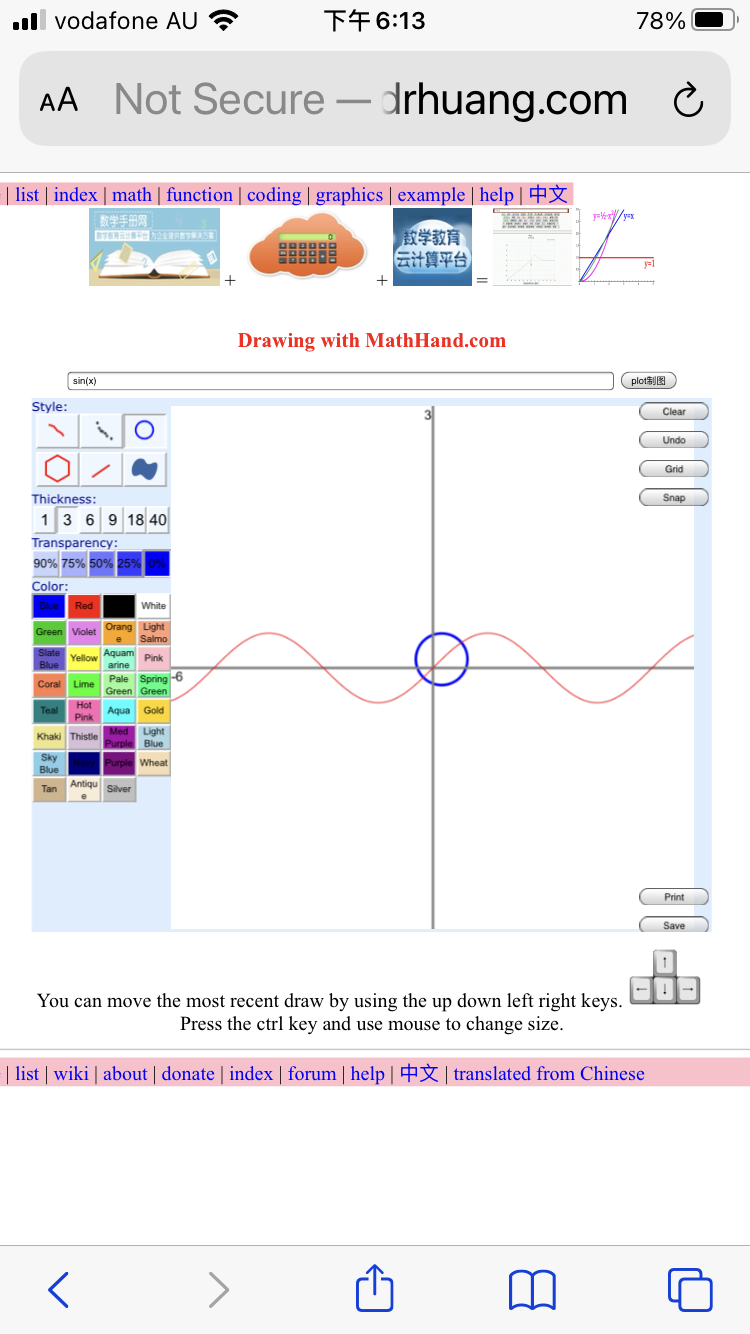
drawing

Next page =>

See Also

Math - Symbol - Handbook - math word
Elementary Math - Higher Math
Calculator - mathHand - mathHandbook
Function - Formula - equation - graphics
Fractional Calculus - differential equation
Tests - Example :

Examples of Fractional Calculus Computer Algebra System 例题

Content

Arithmetic 算术 >>

Exact computation

big number in Java

big number in JavaScript

Round-off errors

Numerical approximations

JavaScript numeric computation

Java numeric computation

Complex 复数

input complex numbers

Convert complex to polar(r,theta) coordinates

convert to vector

complex number plot

complex function plot

Numeric math 数值数学 >>

Algebra 代数 >>

tangent

convert

inverse function

inverse equation

polynomial

Number

Function 函数 >>

Trigonometry 三角函数

Complex Function 复变函数

Complex

References

special Function

Calculus 微积分 >>

Limit

Derivatives

Fractional calculus

differentiate graphically

Integrals

integrator

fractional integrate

numeric computation

numeric integrate

integrate graphically

vector calculus

Equation 方程 >>

Your operation step by step

inverse an equation

polynomial equation

Algebra Equation f(x)=0

absolute equation

Modulus equation

first order equation

second order equation

congruence equation

first order equation:

second order equation:

Probability_equation

recurrence_equation

functional_equation

difference equation

vector equation

2 variables equations f(x,y) = 0

Diophantine equation f(x,y) = 0

2 variables equation f(x,y) = 0 solved graphically on 2D

3D equations

3 variables equation f(x,y,z) = 0

4D equations

system of equations

system of 2 equations

One variable parametric equations x=f(t), y=g(t) on 2D

2 variables parametric equations x=f(u,v), y=f(u,v) on 2D

system of 3 equations

one variable parametric equations x=f(t), y=f(t), z=f(t) in 3D

2 variables parametric equations x=f(u,v), y=f(u,v), z=f(u,v) in 3D

Inequalities

differential equation

ordinary differential equation (ODE)

Your operation step by step

solve graphically

integral equation

indefinite integral equation

double integral equation